Kinematic Analysis
Kinematic analysis is a method used to analyze the potential for the
various modes of rock slope failures (plane, wedge, toppling failures),
that occur due to the presence of unfavorably oriented discontinuities
(Figure 1). Discontinuities are geologic breaks such as joints, faults,
bedding planes, foliation, and shear zones that can potentially serve as
failure planes. Kinematic analysis is based on Markland’s test which is
described in Hoek and Bray (1981). According to the Markland’s test, a
plane failure is likely to occur when a discontinuity dips in the same
direction (within 200) as the slope face, at an angle gentler
than the slope angle but greater than the friction angle along the
failure plane (Hoek and Bray, 1981) (Figure 1). A wedge failure may
occur when the line of intersection of two discontinuities, forming the
wedge-shaped block, plunges in the same direction as the slope face and
the plunge angle is less than the slope angle but greater than the
friction angle along the planes of failure (Hoek and Bray, 1981) (Figure
1). A toppling failure may result when a steeply dipping discontinuity
is parallel to the slope face (within 300) and dips into it
(Hoek and Bray, 1981). According to Goodman (1989), a toppling failure
involves inter-layer slip movement. The requirement for the occurrence
of a toppling failure according to Goodman (1989) is “If layers have an
angle of friction Φj, slip will occur only if the direction of the
applied compression makes an angle greater than the friction angle with
the normal to the layers. Thus, a pre-condition for interlayer slip is
that the normals be inclined less steeply than a line inclined Φj above
the plane of the slope. If the dip of the layers is σ, then toppling
failure with a slope inclined α degrees with the horizontal can occur if
(90 - σ) + Φj < α”.
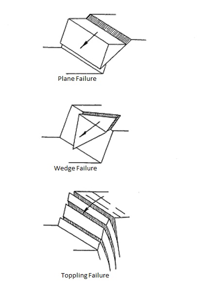
Figure 1: Slope failures associated with unfavorable orientation of
discontinuities (modified after Hoek and Bray, 1981).
Stereonets are used for graphical kinematic analysis. Stereonets are
circular graphs used for plotting planes based on their orientations in
terms of dip direction (direction of inclination of a plane) and dip
(inclination of a plane from the horizontal). Orientations of
discontinuities can be represented on a stereonet in the form of great
circles, poles or dip vectors. Clusters of poles of discontinuity
orientations on stereonets are identified by visual investigation or
using density contours on stereonets (Hoek and Bray, 1981). Single
representative orientation values for each cluster set is then assigned.
These single representative orientation values, can be the highest
density orientation value within a cluster set, or the mean dip
direction/dip of a pole cluster as calculated using equations in
Borradaille (2003).
Great circles for representative orientation values along with great
circle for slope face and the friction circle are plotted on the same
stereonet to evaluate the potential for discontinuity-orientation
dependent failures (Figures 2,3,4) (Hoek and Bray, 1981). This
stereonet-based analysis is qualitative in nature and requires the
presence of tight data clusters for which a reasonably representative
orientation value can be assigned. The chosen representative value may
or may not be a good representation for a cluster set depending on the
tightness of data within a cluster. Tight circular data is more uniform
and has less variation making representative values more meaningful than
for cases where data shows a wide scatter. Fisher’s K value is used to
describe the tightness of a scatter (Fisher, 1953). It is calculated as
follows:
K = M – 1/M-|rn|, where M is no. of data within a cluster, and |rn| is the magnitude of resultant vector for the cluster set (Fisher, 1953).
High K values indicate tightly clustered data, i.e. well-developed
cluster set. If the cluster set is tight, the representative values are
more reliable and so is the stereonet-based kinematic analysis. However,
there are cases when a tight circular clustering of discontinuity
orientations does not exist. A different quantitative approach that does
not require tightly clustered discontinuity sets can be performed by
DipAnalyst 2.0. DipAnalyst 2.0
can also be used for the stereonet-based method.
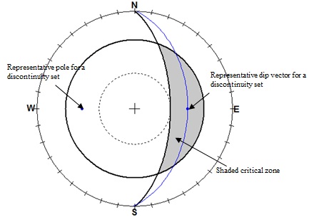
Figure 2: Stereographic plot showing requirements for a plane failure
(Hoek and Bray, 1981, Watts 2003). If the dip vector (middle point of
the great circle) of the great circle representing a discontinuity set
falls within the shaded area (area where the friction angle is higher
than slope angle), the potential for a plane failure exists (figure
created using RockPack).
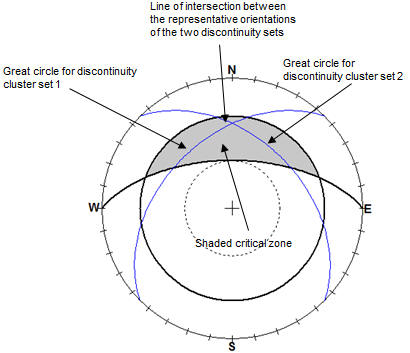
Figure 3: Stereographic plot showing requirements for a wedge failure
(Hoek and Bray, 1981, Watts 2003). If the intersection of two great
circles representing discontinuities falls within the shaded area (area
where the friction angle is higher than slope angle), the potential for
a wedge failure exists (figure created using RockPack software).
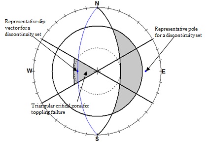
Figure 4: Stereographic plot showing requirements for a toppling failure
(Goodman, 1989, Watts 2003). The potential for a toppling failure exists
if dip vector (middle point of the great circle) falls in the triangular
shaded zone (figure created using RockPack software).
Factor of Safety Calculations
Limit equilibrium analysis is used to calculate the factor of safety
(F.S.) of a slope against failure if the kinematic analysis indicates
the potential for failure. Factor of safety is the ratio of the
resisting forces (shear strength) that tend to oppose the slope movement
to the driving forces (shear stress) that tend to cause the movement
along a plane of discontinuity. The equation for F.S. is:
F.S. = (c +
s
tan
f)/t
(13)
Where: F.S. = factor of safety
c = cohesion
f
= angle of internal friction
s
= normal stress on slip surface
t
= shear stress
According to the limit equilibrium approach, a factor of safety value
equal to 1 represents limiting condition. A value greater than 1
represents a stable slope, and a value less than 1 indicates an unstable
slope. The desired value of factor of safety depends upon the importance
of the slope and the consequences of failure. For heavily travelled
roads, slopes are usually designed to have a factor of safety equal to
or greater than 1.3 under saturated conditions, maximum loads, and worst
expected geological conditions (Canadian Geotechnical Society, 1992;
Wyllie and Mah, 2004). The equations derived for both plane and wedge
failure, consider weight of the sliding block, cohesion along plane of
discontinuity, effect of water present along planes of discontinuity and
tension applied from a rock bolt. Although the equations for factor of
safety calculations of plane and wedge failures are based on Equation
(13), they vary due to differences in the shape of the sliding block for
the case of plane vs. wedge failures. The methods for calculating the
factor of safety for plane and wedge failures with corresponding
equations to determine the resisting and driving forces, including the
effect of water pressure along discontinuities and application of a rock
bolt are given in Hoek and Bray (1981) and Wyllie and Mah (2004).
To calculate factor of safety for plane failure, DipAnalyst 2.0,
requires slope height, slope angle, discontinuity plane inclination,
position and depth of tension crack, and ground water conditions along
the discontinuity plane/tension crack (Figure 5).
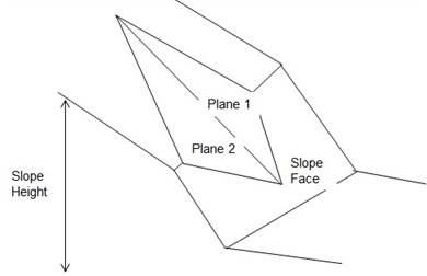
For wedge failure,
DipAnalyst 2.0
follows the “short solution” put forward by Hoek and Bray (1981). The
solution requires slope height, slope angle, orientation of the two
intersecting planes (Figure 6). The “short solution” does not consider
the effect of a rock bolt, and the presence of a tension crack.
Figure 6: Components of wedge failure analysis.
REFERENCES
BORRADAILE, G., 2003,
Statistics of Earth Science Data:
Springer, New York, 351p.
CANADIAN GEOTECHNICAL SOCIETY, 1992, Canadian
Foundation Engineering Manual, BiTech Publishers Ltd.,
FISHER, R.,A., 1953,
Dispersion on a sphere:
Proceedings of the Royal society of London, A217, pp.295-305.
GOODMAN, R. E., 1989,
Introduction to Rock Mechanics:
John Wiley & Sons, New York, NY 562 p.
HOEK, E. and BRAY, J. W., 1981,
Rock Slope Engineering: The
Institute of Mining and Metallurgy, London, England, 358 p.